SpliceV
Installation
Install via pip:
pip install SpliceV
Download source code:
git clone https://github.com/flemingtonlab/SpliceV
Dependencies
- pysam
- matplotlib
- numpy
Tutorial
The minimal requirements for running SpliceV are:
- BAM file
- GTF file
The program will sort and/or index BAM files if this wasn’t done.
The simplest way to plot, using the gene OAS2:
$ SpliceV -b sample1.bam -gtf gencode.v29.basic.annotation.gtf -g OAS2

To filter out low abundance junctions, use the -f flag:
$ SpliceV -b sample1.bam -gtf gencode.v29.basic.annotation.gtf -g OAS2 -f 5

Change the color using the -c flag (can specify hex “#2a9c3c” or RGB or simply, “green”).
$ SpliceV -b sample1.bam -gtf gencode.v29.basic.annotation.gtf -g OAS2 -f 5 -c \#2a9c3c

Plot predicted binding sites for an RNA binding protein (in this case, HNRNPK) with -rnabp. This requires a genome fasta file specified by -fa.
$ SpliceV -b sample1.bam -gtf gencode.v29.basic.annotation.gtf -g OAS2 -f 5 -c \#2a9c3c -rnabp HNRNPK -fa hg38.fa

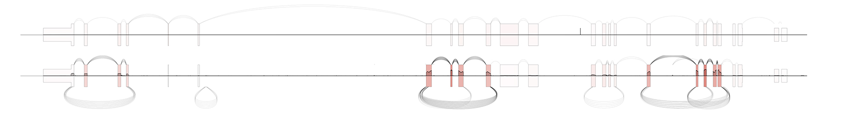
To plot back-splice junctions, if the aligner used outputs chimeric alignments using the ‘SA’ tag (such as STAR v2.5+ using the –chimSegmentMin and –chimOutType WithinBAM), only the bam file is required. Otherwise, use the -bsj flag to point to a file containing junction coordinates and counts (formats described below).
$ SpliceV -b polya.bam rnaseA.bam -gtf gencode.v29.basic.annotation.gtf -g CEP128 -f 5
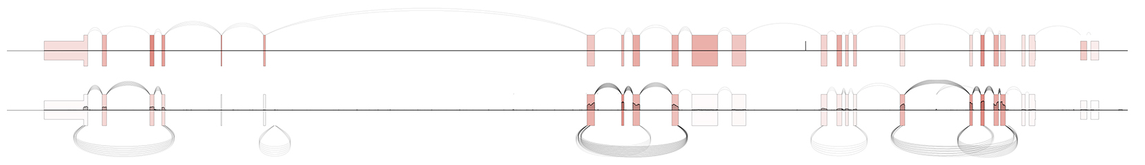
Normalize exon-level expression between samples with the -n flag
$ SpliceV -b sample1_polya.bam sample1_rnaseA.bam -gtf gencode.v29.basic.annotation.gtf -g CEP128 -f 5 -n
Input file formats
Splice junction (-sj) and back-splice junction (-bsj) calls should be tab-separated input files with each line representing the coordinates of one junction in this order: chromosome, smaller coordinate, larger coordinate, strand, counts. Files should contain no header line.
For example:
chr1    123     1234    +       55
chr2    342     53545   -       4
chr2    1000    1200    -       909